A common assumption in time series analysis is that the indicators under study are stationary and could be modeled by a linear model. This would for instance suggest that an indicator would follow the same type of pattern across time with some random fluctuations. The assumption of using constant parameters though, may not be realistic in practice, especially during longer periods of time.
It is common to have time series' which exhibit non-stationary behavior. For instance, gross domestic product (GDP) often shows a linear trend. A common solution is to remove the trend by a transformation such as differencing the indicator or to calculate the growth rate.
Some indicators though, might require performing several differences to make them stationary. In doing so, the intuitive interpretation of them could be lost or might possibly not be as meaningful, such as when the indicator is already in percent.
Time-varying parameter models can ease the strict assumption of constant parameters and give more flexibility. If the underlying process actually follows a time varying process, trying to model it as if it was a constant linear model would also be incorrect.
It is also commonplace for many time series variables to be heteroskedastic, especially financial ones. The shocks a variable exhibit could thus vary with different intensities across time.[1][1]. This could result in forecast intervals being deceptive and thus give misleading results.
For illustrative purposes before diving in to the model, Figure 1 displays the Swedish consumer price index (CPI) between the years 1980-2025 for the under group coffee, tea and cocoa. The variable appears to overall have a positive trend. Observations seem to fluctuate with a different intensity at around the year 2014 and onward compared to the previous years. This could be a sign of heteroscedasticity in the error terms.
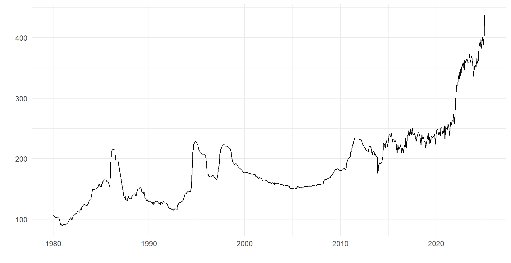
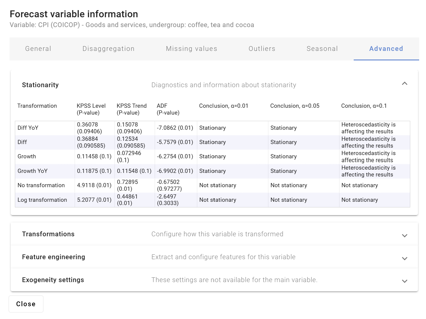
Figure 2 shows the results of different stationarity tests performed by Indicio. As illustrated, the variable is not stationary in levels but it is indicated that it could be stationary by doing some type of transformation. There also seem to be an indication of possible heteroskedasticity and thus that one might be better off modeling this with stochastic volatility.
[1] Or in other words, the variance of the error terms change over time.
The traditional vector autoregression (VAR) with pp lags is of the form
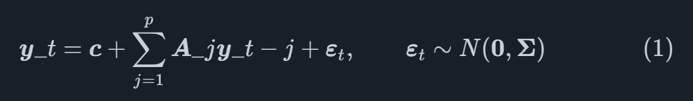
where yt is a vector of K endogenous variables at time t=1,…,T. The model in (1) makes some important assumptions that may not hold for some time series, and can then lead to poor forecast performance. One such assumption is that the VAR coefficient matrices A1,…,Ap and the covariance matrix of the shocks Σ are constant in time. This means for example that the effect of one variable on another variable remains the same during times of rapid economic growth and during a depression, which may not be realistic. The time-varying Bayesian VAR (TVP-BVAR) model relaxes this assumption and allows the parameters in the model to vary over time.
The heteroskedastic case when the covariance matrix Σ changes over time is often of particular interest since it allows the size of the shocks to vary over time. This makes it possible to model the volatility clustering often observed in the data, where there are extended periods of high volatility followed by calmer periods of low volatility. Models with a constant covariance matrix can work poorly in such cases, with forecast intervals that are too wide in calmer periods and too narrow in periods of economic stress. The time-varying Bayesian VAR with stochastic volatility presented below allows the variance covariance matrix of the error term to vary with time, and can therefore be more adapted to handle data with heteroskedasticity.
The time-varying BVAR model (TV-BVAR) is the same model as in (1), but with a time index on the VAR coefficients Aj,t and the covariance matrix of the shocks ΣtΣt to denote that they can now vary over time.
There are three main ways of modeling how the parameters change over time:
This wiki article describes the third type of parameter evolution model, with random walks.
The TV-BVAR model with a random walk parameter evolution can be compactly written as a state-space model (see the technical notes in the Appendix section or Dieppe et al. (2018)):

Equation (2) is referred to as the observation equation, where yt is a vector of endogenous variables, i.e. the main variable along with the other indicators during time t. The design matrix Xt is comprised of all the lagged values of yt, possibly along with an intercept and exogenous variables.
The vector β_t is a stacked version of the VAR coefficients A_1,…,A_K, and is referred to as the latent, unobserved, state vector. The state transition equation (3) models the evolution of the β_t as a random walk. Note how βt varies over time as opposed to a regular VAR model where it would be static through time. It has a recursive form and only depends on the innovation νt with a covariance variance matrix Ω which is assumed to be constant through time. The implication of Ω being constant is that βt changes at the same rate as time goes by. The model for the time evolution of the covariance matrix Σt is described below.
To understand the implication of the TV-BVAR model, consider the following simple univariate special case of the model in (2) and (3) without intercept

where βt could be referred to as the slope of a regression line, a slope that now changes at every time point. The larger variance νt has, the more flexible the model is to capture changes in the parameters over time, but also more prone to overfitting with potentially worse forecasts. Finding the right balance between flexibility and risk of overfitting can be determined from the data by estimating σν2.
There are several ways to model a time varying covariance matrix. The most commonly used model is based on the decomposition

where F is a lower triangular matrix with ones on the diagonal and Λt is a diagonal matrix where the logarithm of the diagonal elements each follow their own autoregressive process with 1 lag. This has two implications. First, since the matrix F is constant over time, the correlation between the variables are taken to be constant and set right from the start. The second implication is that only the variances are allowed to vary over time since Λt is free to evolve over time.
The aim is to compute the posterior distribution of all parameters in the model

where the subscript 1:T denotes a time sequence of data or parameters, for example β_1:T denotes all β_t from t=1 to t=T. The likelihood above is proportional to a normal distribution with mean β_1:T and covariance matrix Σ_1:T. The prior p(β_1:T∣Ω) is also assumed to have a normal distribution and Ω follows an Inverse Wishart distribution a priori. Finally, Σ1:T follows a scaled inverse χ2-distribution.
The analytical solution to obtain the posterior is intractable and a Markov chain Monte Carlo (MCMC) approach using Gibbs sampling is instead used to simulate draws from the posterior distribution in (4). The Kalman filter and smoother are the standard algorithm for inference in state-space models. For time-varying VARs it has been shown however that a more efficient way to sample the time-varying parameters is to draw directly from the multivariate normal distribution of β1:T and to exploit sparsity to make the sampling highly efficient.
The variables are first seasonally adjusted if seasonality is present. Followed by this, several VAR model as in (1) are estimated containing different lags. The number of lags from the model producing the smalles Akaike information criteria (AIC) is then chosen.
After the number of lags to use have been decided, the Time-varying Bayesian VAR is then estimated by using MCMC sampling of the posterior distribution in (4).
Dieppe, A., Legrand, R., and van Roye, B. (2018). The Bayesian Estimation, Analysis and Regression (BEAR) Toolbox Technical guide. Version 4.2 preliminary, European Central Bank.
Statistics Sweden (2025). Consumer price index (cpi) by product group (coicop), 1980=100. month 1980m01 - 2025m02. https://www.statistikdatabasen.scb.se/pxweb/en/ssd/START__PR_ _PR0101__PR0101A/KPICOI80MN/. Accessed: 14.03.2025.

We provide automated forecasting software that blends cutting-edge academic methods with market-specific leading indicators. This helps your organization reach the highest level of forecasting accuracy.
© 2025 Indicio Technologies All Rights Reserved