VECM Lasso

A Vector Error Correction Model (VECM) can be seen as an extension of a VAR model (see Advanced: VAR). Where a VAR model requires all the included variables to be stationary, a VECM does not. Instead, it requires the variables to be cointegrated, meaning that there exists a linear combination of them which is stationary. Just like for a VAR model, including a high number of time series and lags will quickly increase the number of parameters. The risk then becomes that the model will be over-fitted to the data, the VECM lasso remedies this by applying a Lasso penalty to the coefficients of the model.

The first step towards fitting a VECM model is to determine if there is any cointegration present in the data. This is commonly done using the Johansen test which determines the number of stationary linear combinations. These are referred to as cointegration vectors and the number of them as determined by the Johansen test is usually denoted with the letter rr. The VECM Lasso model extends this by applying the Bunea et. al. rank selection criterion which is able to limit the number of cointegration vectors through shrinkage.

From the article on VAR models we have the equations which describes each variable as a function of its own lags and the lags of the other variables as

where the error terms εtεt​ is the part of yt​ which is not explained by the model. In the model there are kk equations, one for each variable. The terms al​ are matrices containing the coefficients at lag l in all equations and yt​ is a vector of the observations of all variables at time t.

In a VECM model, the VAR process is modeled on the first difference transformation of the variables, denoted δt​ at time t. The full VECM model can now be written as

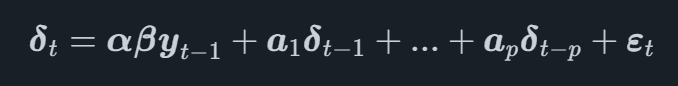
where β is a matrix which contains the coefficients from the cointegration vectors and αα is a matrix which contains the adjustment vectors for the cointegration vectors.

Studying the equation we can see that the first difference of the time series is modeled as a function of the cointegration vectors and the lags of each time series.

The main difference between the regular VECM and VECM Lasso models is that the latter applies a Lasso penalty to shrink the parameters towards zero, similar to what a VARX Lasso (Advanced: VARX Lasso) model does as contrasted to a regular VAR model.

How does Indicio fit a VECM Lasso model?

To fit a VECM Lasso model, the first task is to select the maximum order (i.e. the maximum number of lags) of it. In Indicio this is done by fitting VAR models of order 1,...,pmax⁡​ where ⁡p max​ is the maximum number of lags selected by the user. The one that fits the data the best according to Akaike's Information Criterion (AIC) is selected, this favors a simple model over a more complicated one, but still accounts for a good model fit.

After the lag order is selected, the Bunea et. al. rank selection criterion is applied to determine the cointegration rank rr.

With these parameters selected, the next step is to split the data into two parts, say that we have a time series YY with NN observations. The first part contains observations 1 to ntrainntrain​ where the latter is the number of observations used to fit the initial model, this is called the training set. The second part contains the remaining data containing n test=N−ntrain​ observations.

The second step is to to fit models using the training set of observations for an array of different λ values. These models are then used to create a forecast starting at the first point in the test set. The models are then adjusted to use one more observation of the test set when fitting, and a forecast is made, starting one point further ahead in time than the previous. This way a large number of back-test forecasts are created which emulate building models at previous points in time and making a forecast.

Comparing the back-test forecasts with the actual outcome in the data, mean squared forecast error (MSFE) values can be calculated for the different values of λ, providing a measure of how well the model performs in a forecasting scenario given a specific λ value.

With the optimal λ value selected, a final model which is fitted to all the data is created using that value. This results in a model with a penalty that is tuned to extract the maximum predictive power of the data, without over-fitting the model.

‍