MIDAS Sparse Group Penalty

The Mixed Data Sampling Sparse Group Lasso (MIDAS Sparse Group Lasso) model is one of the mixed frequency models available in Indicio. It is similar to the MIDAS Lasso model, but instead of using the basic Lasso penalty, it is using a sparse group Lasso which is tailored to the structure of the data.

When forecasting a slower moving time series such as a monthly, quarterly or yearly one, there can be a great benefit to use high frequency indicators to provide more up to date information about how what is happening in the economy.

The most basic MIDAS model is the one referred to as Unrestricted MIDAS which in the case of a quarterly main variable with a single monthly indicator will take on the form

where the indicator variable has the subscript t,mi​ where mimi​ is referring to the i'th latest monthly observation available. For example, if we were to forecast Q2 and we have monthly data of the indicator available up until May, we would add the observations of March, April and May into the equation.

In some cases we may have a quarterly or even a yearly main variable, and perhaps weekly or even daily indicators. This results in a very large number of parameters to be estimated, which may both make the estimates unstable and increase the risk of over-fitting the model to the data. The MIDAS Sparse Group Lasso model solves this by applying a Group Lasso penalty when fitting the model.

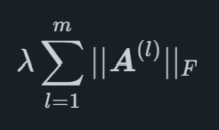
Mathematically, the Lasso Sparse Group penalty is a term which is added to the function which is optimized when fitting the model, for a general regression model with pp coefficients it can be written as

where and ∣∣X∣∣2​ is the Frobenius norm of X which is defined as

for a matrix X, where the tracetrace is the sum of diagonal entries of a square matrix. The benefit of this type of penalty is that it is able to shrink whole groups of coefficients to zero, leaving other groups with non-zero values. For the MIDAS Sparse Group Lasso this is used to be able to penalize all the lags of specific variables as groups, allowing the model to select the optimal effect a specific variable should have on the main variable.

How does Indicio fit a MIDAS Sparse Group Lasso?

The first step towards fitting a MIDAS Sparse Group Lasso model is to split the data into two parts which are referred to as the training set and the testing set.

The second step is to to fit model using the training set of observations for an array of different λ values. These models are then used to create forecasts for the time points in the test set. This process is repeated multiple times, and the average forecast error is used as a measure of how good the model performs given different values of λ. From this the best value giving the most accurate forecasts is selected.

With the optimal λ value selected, a final model which is fitted to all the data is created using that value. This results in a model with a penalty that is tuned to extract the maximum predictive power of the data, without over-fitting the model.

‍