An ARIMA model consists of three distinct parts, namely Autoregressive (AR), Integrated (I) and Moving Average (MA).
An autoregressive model describes the current value as a function of a fixed number of past values (lags). Denoting the current value at time tt as Yt, a simple autoregressive model with pp lags is written as
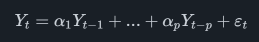
where αi is the coefficient for lag i and εt is the error term (i.e. the variation that the model does not explain at time tt). As an example, if our variable Yt represents sales at time period tt, the model above assumes that sales in the current month is a function of sales in the pp previous months.
The integrated part of the model indicates that the data is replaced with the difference between each value and the value prior to it. The differenced values can be written as

Combining this with an autoregressive model means that if we in the example above were modelling sales directly, we are now instead modelling the difference in sales from period to period as a function of the pp previous differences. A model can be integrated of a higher order, where the differences are taken multiple times.
Finally, the moving average part is modelling the error terms εtεt as a linear combination of the previous error terms. This can for qq lags be written as
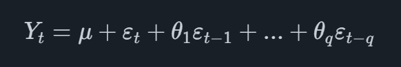
where μ is the mean of the data and θi is the coefficient in the linear combination for lag i. This can be thought of as a weighted moving average over the last q periods. If we again consider the sales data example, the moving average model considers sales at period t to be a weighted average of the q last periods, plus a random error εt.
Putting these three components together, we get the ARIMA model which is quite flexible in that it can model a lot of different time series. When discussing an arima model it is quite common to describe it using the order it has, meaning which values p and q in the AR and MA parts have, and how many times d it is integrated. We write that we have an ARIMA model or order (p,d,q)(p,d,q). The values of these three parameters determine the shape of the model.
We can write the full ARIMA (p,0,q)(p,0,q) model as
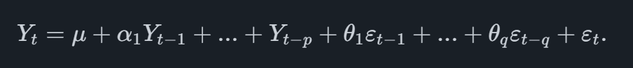
If an integration order other than 0 is used, the Yt values are replaced with δt accordingly on both sides of the equation.
In Indicio, it is possible to add events to a forecast, these are modeled as exogenous variables which means that they follow a predetermined path, even in the unknown future periods of the forecast. An ARIMA model supports these by adding them on the right hand side of the equation, meaning that the current value is not only a function of its own past lags, but also of the contemporary values of the exogenous variables. If an extreme event had an effect on the data, an event at this point in time will allow the model to assign the part of the data that is not explained by the model using the event, giving the model a better opportunity to describe the time series as it would have looked without the event.
To fit an ARIMA model, the parameters p,d and q must be selected. In Indicio this is done by evaluating a large number of different models. The one that fits the data the best according to Akaike's Information Criterion (AIC) is selected, this favors a simple model over a more complicated one, but still accounts for a good model fit.

We provide automated forecasting software that blends cutting-edge academic methods with market-specific leading indicators. This helps your organization reach the highest level of forecasting accuracy.
© 2025 Indicio Technologies All Rights Reserved